Machine Learning But Funner 02 - The (Simplified) Theory of Convolutional Neural Networks

Today I aim to cover the basic theory of convolutional neural networks in the most high level fashion I can, ignoring (or as we computer scientists like to lie to ourselves: abstracting away from) most of the maths, targeting this tutorial at complete beginners. However I will mention as an obligatory disclaimer now that in order to gain a deeper understanding of the topic i.e. to build a CNN from scratch, I will do as every blogger and direct you to an over-detailed book: Artificial Intelligence for Humans Volume 3: Deep Learning and Neural Networks which covers the topic in Chapter 10.

Network Structure

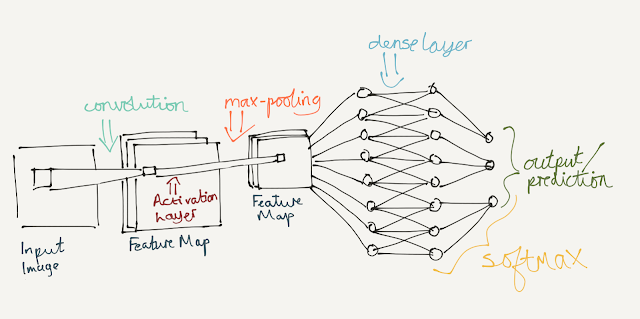
The CNN model is built on top of the usual feed-forward neural network model and so the structure is similar to what you may be comfortable with already, except the 'hidden layer' will be replaced by the layers below:

• Convolutional Layers
• Pooling Layers (here we will use max-pooling but there are others)
• Dense Layers (this is often the same as a regular output layer in feed-forward networks)

In a structure like so:

Convolution

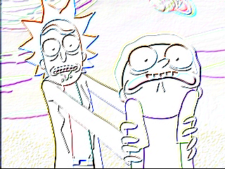
Here you will see that the input image is scanned over by a grid, and passed as input to the network. The network then applies one layer of convolution to the input image, which involves splitting the image into a 3D cube-like structure containing 3 frames each representing the red, green and blue information of the image separately. After doing so it applies a number of convolutional filters (sometimes called neurons) to the image. You can read more about these here, but they are effectively the same as just applying a certain photoshop filter (or in maths terms, a matrix) to image data to highlight certain features e.g. a Roberts cross edge enhancing filter on this famous artist interpretation of Doc and Marty:

So I hope you can see now how a network with 100+ different filters will have the ability to pick up significantly complex features which greatly improves its ability to recognise real world things like dogs and moon-men. Once the network has applied the convolutional filter to the image we are left with what is called a feature/activation map. A feature map corresponds to the activation of a given neuron on a given input area. Imagine we apply the edge detection filter to the image on the left, note how the activation map looks on the right:

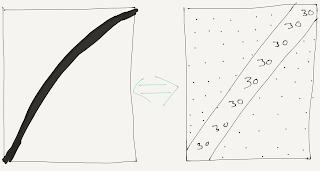
Here, the dots represent rows of 0's (indicating there is nothing in that area which may be an edge) however the '30' values in the 2D array indicate a high likelihood of an edge existing in that image area.

Activation Layer

Now let's move past what feels like a dragged out and simplified image processing lecture to the machine learning! Now we have our activation map we must apply an activation function to it, in this example we will use ReLU (Rectified Linear Units) due to it being the preferred activation function in research however some still say that the sigmoid function or hyperbolic tangent will provide the best training results. I am not one of those people. Now, the idea of an activation layer is to introduce non-linearity into the system, as this improves generalisation of the inputs and outputs. The function ReLU(x) just returns max(0, x) or simply, it removes negative weights in the activation maps.

Pooling Layer

Following our activation layer, it is normally best practice to apply max-pooling (or any other kind of pooling) to the feature map. Max-pooling layers are sometimes referred to as downsampling layers. The theory behind a max-pooling layer is to scan over the image in small grids, replacing each grid with a single cell containing the highest value in the given grid:

The reason for this is that once we know a given feature is in a given input area, we can abstract away the exact location of that feature for the sake of generalising the data to minimise over-fitting (which is kind of like knowing what the side of a dog looks like but not being able to spot it from head-on). An example of this is when your training accuracy is 99% but when you test it on unseen data it get's 50% accuracy.

Output Layer

Following the max-pooling layer, we are left with another activation map, which is passed to what is often referred to as the fully connected part of the network, containing a dense layer which simply maps the output of every neuron in the previous layer to a neuron in the dense layer (a.k.a. a linear map) and applies the softmax function to the outputs, which is another activation function like our ReLU function before. Here we use softmax because we will be using our neural network to classify images, and a softmax allows our outputs to be returned as a list of probabilities summing to 1, each probability representing the probability a given image belongs to a given output class, but later when we cover pixel prediction and in-painting, we will use a linear activation function here.

Note here how we have only used one convolutional layer and one pooling layer, to achieve best accuracy these are often stacked sequentially with multiple of them (as in deep learning if you hadn't got it yet), and after each full iteration to the output layer we have what is called back-propagation where we go backwards through the network and update our weights according to our calculated loss (basically how well our model predicted the output), often using stochastic gradient descent or some other optimisation algorithm.

Summary

What to take away for the next tutorial:

• A CNN is similar in structure to a RNN, except designed with image recognition in mind
• CNNs have 3 common layer types: convolutional, pooling and dense
• Convolutional layers apply filters/neurons to images to highlight features
• A feature map represents how likely it is that an input image contains a given feature
• Pooling allows us to generalise our data and minimise over-fitting
• Optimisation in a CNN is done just like a regular old feedforward network

That's the end of the theory lesson, and in the next post we will get our hands dirty with some TensorFlow CNN examples, including implementing a gesture classifier which should be able to classify happy, sad, sleepy, surprised, and winking gestures in a given image. Prepare your coding fingers boys and girls, it's going to get hack-y!